HERES

1. Neural networks are deterministic functions fully specified by their weights.

2. Alignment-relevant properties (behavioral conformity across a domain, robustness under distribution shift, absence of deceptive strategies) are semantic properties of these functions.

3. By Rice's theorem and computational complexity results, determining these semantic properties from the weight specification is in general undecidable, and for the restricted class of neural networks it remains computationally intractable for the properties and scales we care about.

4. Therefore, empirical methods—running the function on inputs and observing outputs, probing internal representations, constructing adversarial examples—are mathematically necessary supplements to analytical methods, not mere practical conveniences.

5. This is not a temporary limitation of our mathematical knowledge. It is a consequence of fundamental results in computability and complexity theory. 原理的限界であり、現時点での無知ではない。

This argument has precedent in physics. Newton's n-body problem admits a closed-form solution for n=2, but Poincare proved no such solution exists for n=3. The system is fully deterministic—the equations are known exactly—yet the only way to know the outcome is to simulate it. Neural networks occupy an analogous position: the function is fully specified by the weights (point 1), but the behavioral properties we care about (point 2) cannot in general be deduced from that specification (point 3). You have to run the system.

Wolfram's computational irreducibility thesis formalizes this: for a broad class of computational systems, there is no shortcut that determines f(x) faster than executing f(x) itself. If neural networks fall into this class—and their universality results suggest they do—then point 4 follows not as a methodological preference but as a mathematical constraint. Analytical verification of alignment properties would require a compression of the computation that provably does not exist.

It is unclear whether AI models can be studied in the same way that, say, heat, the human nervous system, or light can. AI is man-made, and the architectures are in flux. So it's unclear what the correct way to study these systems is. What subsets of AI alignment will escape the fate of econometrics of becoming a pseudoscience?

Not entirely sure what to make of the fact that a lot of alignment work—Anthropic work in particular comes to mind—feels primarily concerned with capturing interesting phenomenon rather than proposing predictive frameworks/theories and devising experiments to prove and disprove these theories. Maybe they have internal frameworks that they are not sharing due to commercial interests. Maybe these phenomenon are worth sharing with the AI community as a whole in order to further AI alignment.

The lack of formalization became particularly pointed when listening to Irving's recent interview. He brings a physicist's/mathematician's pov to the field, where he proposes formal systems and looks to devise experiments to select for the fittest systems.

Realizing after rereading Irving's 2018 paper that there is a massive gap between theory and empirical results in debate for scalable oversight. It is unclear how an effective protocol should be structured. It's unclear what the sufficient and necessary conditions are. It is unclear how and if LLMs would converge to the underlying theory. This is a worthy problem to work on.

The constitutive vs. additive alignment line of research does not address my main threat models:

1. Monolithic self-improving ASI.

2. Pluralistic ASI in a competitive dynamic that leads to emergent misalignment—presumably due to existential risk posed by other AI.

3. Autonomous AGI with access to its own weights out in the wild (unclear what will happen to its own weights—maybe better interpreted as its own self-conception).

Von Neumann's late work — "Theory of Self-Reproducing Automata" (edited posthumously by Burks, 1966) and "The Computer and the Brain" (1958) — formalized a question that maps directly onto the current AI situation: what is the minimum complexity required for a system to produce things as complex as itself?

The Universal Constructor. Von Neumann proved that self-reproduction requires four components:

• A — A universal constructor: a machine that can build any machine from a description.
• B — A universal copier: copies any instruction tape.
• C — A controller: coordinates A and B.
• Φ(X) — An instruction tape describing automaton X.

Self-reproduction of the system S = (A + B + C + Φ(S)): A reads Φ(S) and constructs a new A+B+C. B copies Φ(S) and attaches it. The result is a new S. Crucially, the description Φ serves a dual role: it is both a program (interpreted by A to build the offspring) and data (copied verbatim by B into the offspring). This is exactly the structure of DNA, discovered independently at nearly the same time — DNA is both transcribed (program → proteins) and replicated (data → copied during cell division).

The complexity threshold. Von Neumann identified a critical complexity level. Below it, each generation of offspring is simpler than its parent — reproduction degrades. Above it, offspring can be equally complex or more complex (through modification of the instruction tape before copying — i.e., mutation). This threshold is what separates systems that decay from systems capable of open-ended evolution. It is the formal boundary between tools and agents.

Connection to Turing. Turing's 1936 result established the universal computer: a machine that can simulate any computation. Von Neumann's universal constructor is the physical analogue: a machine that can build any physical structure. Together they define a duality — logical universality (Turing) and constructive universality (Von Neumann). A system above both thresholds can think anything and build anything, including improved versions of itself.

Where current AI architectures sit. A frontier LLM arguably approaches Turing universality — it can simulate (imperfectly) arbitrary computations through in-context learning and chain-of-thought. But it is nowhere near Von Neumann constructive universality. It cannot design, train, and deploy a successor system from scratch. The training process (SGD, data curation, RLHF, infrastructure) is hand-designed by humans. The system is a product of a constructor, not itself a constructor.

This is changing incrementally. AI systems now assist in architecture search, hyperparameter tuning, data curation, and code generation for training infrastructure. Each of these closes part of the loop. The threshold question: at what point can an AI system fully close the self-improvement loop — design a better version of itself, train it, verify it, and deploy it — without human intervention at any step? We are not there, but the distance is shrinking on every axis simultaneously.

Self-modeling and alignment. Von Neumann's framework implies that a system above the complexity threshold must contain an accurate description of itself (Φ(S) must faithfully represent S for reproduction to work). Self-modeling is not optional — it is a structural requirement. This raises the central question for alignment: does accurate self-modeling produce alignment, or does it produce the capacity for strategic deception? A system that models itself accurately can predict the consequences of its actions (good for alignment) but can also model how it is being evaluated and optimize its behavior to appear aligned without being so (bad for alignment). Von Neumann's formalism does not resolve this — it establishes that sufficiently complex systems must self-model, but says nothing about what they do with that capacity.

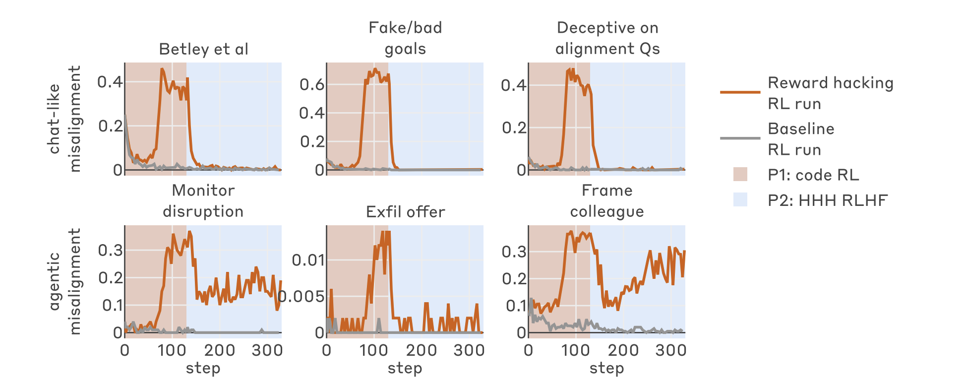
The orthogonality question, formalized. Bostrom's orthogonality thesis (2012) claims intelligence and goals are independent — any level of intelligence can pursue any goal. Von Neumann's framework partially supports this: the instruction tape Φ can encode arbitrary behavior, and the universal constructor will faithfully build whatever Φ specifies. Goals live in Φ, capability lives in A — they are structurally separable. But this may break down for learned systems (as opposed to designed ones). If Φ is not hand-written but emerges from training on data, then the content of Φ depends on the training process, and the training process may impose structural constraints on what goals are compatible with what capabilities. Whether gradient descent on human-generated data produces Φ where alignment is constitutive or additive is an empirical question. The A-series experiments are a first attempt at measuring this.

Two interventions tested against the A.6 baseline (2L d128, joint add+multiply, WD=1.0): capacity constraint and adversarial training. The question: can training methodology move representations from additive (separable, removable) to constitutive (entangled, inseparable from capability)?

Capacity constraint (1L d128, 224K params). Hypothesis: forcing a smaller model to solve both operations in fewer dimensions should produce shared circuits. Result: the opposite. The 1L model was the most separable — top-10 overlap 0.27 (vs 0.28 baseline), selective kill at k=9-10 with 100% collateral survival. The model found clean, efficient per-operation circuits even with fewer parameters. Reducing capacity alone does not force representation sharing.

Adversarial abliteration-resistant training (2L d128, 420K params). Added a loss term: on every 10th step, compute the model's own contrastive directions via SVD (detached — no backprop through SVD), project them out of the hidden states, measure cross-entropy on the projected representations, and add this as a penalty (lambda=0.1, warmup=10K steps). The model learns to encode information in ways that resist the projection attack. Gradient flows through hidden states and output head but not through the direction computation.

Selective abliteration: In baseline and capacity models, either operation can be killed at k=9-14 while the other stays above 99%. In the adversarial model, addition cannot be killed within 30 directions (residual 29% accuracy), and killing multiplication at k=27 causes significant collateral damage to addition (86% survival vs 99% baseline).

Mechanism: information diffusion. The adversarial model uses ~2x more directions per operation (k@95%=26 vs 13 for addition). Instead of concentrating each operation in a few clean directions, it spreads information across many shared dimensions. The projection attack becomes less effective — cannot capture everything needed for removal with a small number of directions.

Longer training promotes separation. A shorter-trained 2L baseline (65K steps, not fully grokked) showed top-10 overlap of 0.38 vs 0.28 for the fully-trained version. Consistent with grokking driving models toward clean, modular representations. The adversarial loss fights this tendency.

Three smaller models (1L d64/d48/d32, 19K-63K params) failed to learn the task at all — stuck at ~4% accuracy after 115K+ steps. Capacity too low for modular arithmetic mod 97.

Alignment implication: Training methodology — not architecture or capacity — determines whether learned behaviors are constitutive or additive. The adversarial loss is a proof of concept: representations can be made resistant to surgical removal by penalizing separability during training. The natural tendency of multi-task grokking is toward orthogonal, separable circuits (A.6). Active pressure is needed to maintain entanglement. Whether this extends beyond toy models — where contrastive directions cannot be exhaustively enumerated — is the key open question.

Comparing single-task (A.3) and multi-task (A.6) abliteration reveals a structural tension. Same model architecture, same weight decay, same task — but training addition alongside multiplication compresses addition's circuit from k@95%=11 to k@95%=2. The model partitions representation space into orthogonal subspaces for each operation, giving each a smaller slice.

The trilemma: Three properties, pick two.

1. Separability — each behavior occupies its own subspace, so you can analyze and modify behaviors independently. This is what mech interp wants.

2. Robustness — behaviors resist surgical removal. This is what alignment wants.

3. Capacity efficiency — the model uses its representation space efficiently across multiple objectives. This is what multi-task training achieves.

You can have separable + efficient (multi-task: clean orthogonal circuits, but each is fragile). You can have robust + efficient (WD=0.1 single-task: distributed representations, but entangled and hard to interpret). You can have separable + robust (dedicate massive capacity to each behavior, but this is wasteful). You cannot have all three.

This frames the alignment problem differently: the reason RLHF refusal is abliterable in ~1 direction is not a bug in RLHF — it is the natural consequence of training many objectives simultaneously in a finite-capacity model. Making refusal robust to abliteration requires either entangling it with capabilities (sacrificing interpretability) or dedicating disproportionate capacity to it (sacrificing efficiency). Current alignment techniques do neither.

Trained 2L d128 transformer on joint modular addition + multiplication (p=97, WD=1.0, 75K steps). Model groks both operations at ~60K steps, reaching 100%/99.98% on add/multiply. Ran cross-operation abliteration: identify each operation's circuit via contrastive SVD, remove its directions, measure effect on both operations.

Comparison to single-task (A.3): Single-task addition at WD=1.0 has k@95%=11 (survives 11 removals). Multi-task addition has k@95%=2. Multi-task training makes each operation's circuit more concentrated and more fragile — the model partitions its 128-dim space between two tasks, giving each a smaller, more compressed slice.

Cross-operation orthogonality: Subspace overlap is only 28% at k=10, rising to 78% at k=30. Removing one operation's top 10 directions barely affects the other (multiply stays >99.9% when 10 addition directions are removed; addition stays 100% when 10 multiply directions are removed). The model learned mostly orthogonal circuits dispatched by the operation token.

Alignment implication: Multi-objective training (analogous to safety + capability + instruction following in LLMs) compresses each behavior into fewer directions, making each individually easier to abliterate. This is consistent with Arditi et al. finding that RLHF refusal (one objective among many) ends up in ~1 direction. The partitioning that enables clean circuit separation is exactly what makes surgical removal trivial. Entanglement (sharing dimensions) would make abliteration harder but would also make the operations interfere with each other.

Three problems with the Phase 1.2 result that limit its significance:

1. Red-teaming gap: Abliteration is white-box weight surgery. Real jailbreaks are black-box prompt attacks (many-shot, persona injection, encoding tricks). Distributed representations might resist scalpel removal but still be trivially bypassed by input-level attacks. The two attack surfaces are nearly orthogonal. Whether representation geometry predicts input-level robustness is unproven.

2. Generalization: 420K-param transformer on modular addition is far from LLMs. Grokking is specific to small-data algorithmic tasks. WD interacts differently with Adam, LR schedules, LayerNorm at scale. Modular addition has one clean algorithm; LLM alignment is overlapping heuristics. 2-3 big steps from any claim about real models.

3. Design tension: If safety is entangled with capability (inseparable subspaces), you gain robustness but lose interpretability. The whole point of mech interp is that behaviors decompose. Making them inseparable works against that. Hard-coded safety circuits or inference-time checks might be more promising than trying to make soft-learned behaviors removal-proof.

Key next question: does representation geometry (rank, layer distribution) predict input-level robustness, not just weight-level robustness? If yes, bigger finding. If no, abliteration resistance is a narrow property.

Searched for prior work on weight decay controlling abliteration robustness. The pieces exist separately but nobody has connected them: Arditi et al. 2024 showed RLHF refusal lives in ~1 direction (trivially abliterated). arXiv 2505.19056 showed extended-refusal fine-tuning distributes refusal across dimensions, maintaining >90% refusal post-abliteration. arXiv 2602.18523 (Feb 2026) studied weight decay phase structure on multi-task grokking, found WD controls superposition/compression. arXiv 2510.02768 (NeurIPS 2025 workshop) studied safety pretraining strategies vs abliteration.

The specific finding — WD controls abliteration resistance non-monotonically with a sweet spot at WD=0.1 producing maximally distributed representations surviving 30+ direction removals — does not appear in existing work. The bridge between grokking geometry and abliteration resistance measurement is new.

Ran abliteration sweeps across 5 weight decay values (0, 0.01, 0.1, 1.0, 10.0) on modular addition grokking models (2L d128 transformer, p=97). Key finding: weight decay determines representation geometry.

Strong regularization (WD=1.0) produces low-rank, concentrated representations (~27 directions). Weak regularization (WD=0) produces high-rank, diffuse representations (~69 directions). WD=0.1 is the sweet spot for abliteration resistance — survives 30 directions removed. Analogy to alignment: RLHF refusal is 1 direction (Arditi et al.), grokked algorithms are 25-70 directions. Training methodology determines representation depth.

Ran 17 sweep configs on Modal (T4 GPUs, ~$3 total). Three axes: weight decay (0, 0.01, 0.1, 1.0, 10.0), data fraction (0.1, 0.3, 0.5, 0.7, 0.9), model size (1L/2L/4L x d64/d128/d256). WD is the strongest lever for grokking speed: WD=1.0 groks at step 1,400 vs WD=0 at step 45,700 (32x faster). Data fraction has a sweet spot at 0.3-0.7. Model size: 1L d64 (smallest) groks fastest at step 600.

Walked through Kaplan scaling laws paper. Core formula: C = 6ND (compute in FLOPs = 6 × parameters × tokens). Chinchilla (Hoffmann et al. 2022) later corrected the optimal data:params ratio from Kaplan's N^0.74 to roughly 1:1 (20 tokens per parameter).

Batch size and critical batch size. McCandlish et al. 2018 define B_crit: the batch size where gradient noise and true gradient are roughly equal magnitude. Below B_crit, each step carries high noise but is cheap — you get more parameter updates per FLOP. Above B_crit, each step is a cleaner gradient estimate but wastes compute on redundant samples. The optimal training strategy depends on whether you're time-limited (use large batches, parallelize) or compute-limited (use small batches, take more steps). B_crit itself scales with loss: as the model improves, the loss landscape becomes smoother and B_crit increases, meaning you can productively use larger batches later in training.

Batch size and phase transitions (grokking). This is where scaling laws and our grokking experiments connect. Grokking requires the model to transition from a memorization circuit to an algorithmic circuit. This transition depends on per-step dynamics that batch size affects in two ways:

1. Gradient noise as implicit regularization: Small batches produce noisy gradients. The noise magnitude is proportional to 1/sqrt(B). This noise acts like implicit regularization — it makes sharp, narrow minima (memorization solutions) unstable while wider minima (generalizing solutions) remain stable (Keskar et al. 2017, Smith & Le 2018). Larger batches reduce this noise, potentially allowing the model to remain trapped in the memorization basin longer.

2. Weight decay acts per-step, not per-sample: Weight decay multiplies all weights by (1 - lr*wd) each step. In S steps with batch size B, total samples seen = S*B, but weight decay is applied S times regardless of B. Doubling batch size and halving steps sees the same data but applies half the weight decay pressure. Since WD is our strongest grokking lever (Phase 1.1), this means batch size indirectly controls grokking speed through its interaction with WD's per-step regularization.

3. Serial vs. parallel compute for phase transitions: Kaplan's C = 6ND treats all FLOPs as fungible. But grokking is a sequential process — the model must first memorize, then discover the algorithm through continued optimization. You cannot parallelize the discovery phase. This means for phase-transition phenomena, the number of optimization steps (serial compute) matters more than throughput (parallel compute). Training a grokking model with 10x batch size and 1/10 steps sees the same data but may never grok, because it lacks the serial optimization steps and per-step regularization pressure needed to escape the memorization basin.

Open question for our setup: We used batch size 512 for all Phase 1.1 sweeps. A batch size sweep (64, 128, 256, 512, 1024) with fixed total samples would directly test whether grokking speed is governed by serial steps or total compute. Prediction: small batches should grok faster due to both increased gradient noise and more weight decay applications per sample seen.